After running the pipeline
Snakemake report
We have also automatically generated a general report for the workflow, which is stored in tutorial/ subfolder relative to the working directory of the pipeline. Take a look at the statistics in report.html. Some rules took longer to complete than others, but they were still very fast.
Throughout the pipeline, several simple plots are generated to give insights into the insertions' characteristics, such as their length and chromosomal specificity. Navigate to the results tab to explore the detected insertion lengths. It appears that some reads only contain parts of the insertion.
If you would like to explore quality control metrics, check out the multiqc.html report in the results tab. Since our data is simulated, you will probably not be too happy with it.
Output directory structure
Now, let's examine the output files directly generated by the pipeline. Navigate to the output folder as specified in the config. To get an overview of the file structure in this directory, run tree tutorial/out/simulation_tutorial/.
Output directory structure
tutorial/out/simulation_tutorial/
├── config_settings.yml
├── final
│   ├── functional_genomics
│   │   ├── Functional_distances_to_Insertions_S1.bed
│   │   └── Functional_distances_to_Insertions_S2.bed
│   ├── localization
│   │   ├── ExactInsertions_S1.bed
│   │   ├── ExactInsertions_S2.bed
│   │   ├── Heatmap_Insertion_Chr.png
│   │   ├── Insertion_length.png
│   │   ├── InsertionPoints_S1.bed
│   │   └── InsertionPoints_S2.bed
│   └── qc
│       ├── Fragmentation
│       │   ├── Insertions
│       │   │   ├── insertions_100_S1
│       │   │   │   ├── 100_fragmentation_distribution.png
│       │   │   │   └── 100_read_match_fragmentation_distribution.png
│       │   │   └── insertions_100_S2
│       │   │       ├── 100_fragmentation_distribution.png
│       │   │       └── 100_read_match_fragmentation_distribution.png
│       │   ├── Longest_Interval
│       │   │   ├── S1
│       │   │   │   ├── Longest_interval_Read-343.png
│       │   │   │   ├── Longest_interval_Read-555.png
│       │   │   │   ├── Longest_interval_Read-561.png
│       │   │   │   ├── Longest_interval_Read-745.png
│       │   │   │   └── Longest_interval_Read-902.png
│       │   │   └── S2
│       │   │       ├── Longest_interval_Read-262.png
│       │   │       ├── Longest_interval_Read-417.png
│       │   │       ├── Longest_interval_Read-522.png
│       │   │       ├── Longest_interval_Read-682.png
│       │   │       └── Longest_interval_Read-824.png
│       │   └── Reference
│       │       ├── reference_100_S1
│       │       │   └── 100_fragmentation_distribution.png
│       │       └── reference_100_S2
│       │           └── 100_fragmentation_distribution.png
│       ├── mapq
│       │   ├── Insertions_S1_mapq.txt
│       │   ├── Insertions_S2_mapq.txt
│       │   ├── S1_mapq_plot.png
│       │   └── S2_mapq_plot.png
│       └── multiqc_report.html
└── intermediate
    ├── blastn
    │   ├── Coordinates_100_InsertionMatches_S1.blastn
    │   ├── Coordinates_100_InsertionMatches_S2.blastn
    │   ├── Filtered_Annotated_100_InsertionMatches_S1.blastn
    │   ├── Filtered_Annotated_100_InsertionMatches_S2.blastn
    │   ├── Readnames_100_InsertionMatches_S1.txt
    │   ├── Readnames_100_InsertionMatches_S2.txt
    │   └── ref
    │       ├── Filtered_Annotated_100_InsertionMatches_S1.blastn
    │       └── Filtered_Annotated_100_InsertionMatches_S2.blastn
    ├── fasta
    │   ├── fragments
    │   │   ├── 100_Insertion_fragments.fa
    │   │   ├── 100_Insertion_fragments.fa.ndb
    │   │   ├── 100_Insertion_fragments.fa.nhr
    │   │   ├── 100_Insertion_fragments.fa.nin
    │   │   ├── 100_Insertion_fragments.fa.njs
    │   │   ├── 100_Insertion_fragments.fa.not
    │   │   ├── 100_Insertion_fragments.fa.nsq
    │   │   ├── 100_Insertion_fragments.fa.ntf
    │   │   ├── 100_Insertion_fragments.fa.nto
    │   │   └── Forward_Backward_Insertion.fa
    │   ├── Full_S1.fa
    │   ├── Full_S2.fa
    │   ├── Insertion_S1.fa
    │   ├── Insertion_S2.fa
    │   ├── Isolated_Reads_S1.fa
    │   ├── Isolated_Reads_S2.fa
    │   ├── Modified_S1.fa
    │   └── Modified_S2.fa
    ├── functional_genomics
    │   ├── Annotation_ucsc_genes_Insertions_S1.bed
    │   └── Annotation_ucsc_genes_Insertions_S2.bed
    ├── localization
    │   ├── ExactInsertions_S1.bed
    │   ├── ExactInsertions_S2.bed
    │   ├── Sorted_InsertionPoints_S1.bed
    │   └── Sorted_InsertionPoints_S2.bed
    ├── log
    │   ├── detection
    │   │   ├── BAM_to_BED
    │   │   │   ├── Postcut_S1.log
    │   │   │   ├── Postcut_S2.log
    │   │   │   ├── Precut_S1.log
    │   │   │   └── Precut_S2.log
    │   │   ├── basic_insertion_plots
    │   │   │   ├── heat.log
    │   │   │   └── length.log
    │   │   ├── build_insertion_reference
    │   │   │   └── out.log
    │   │   ├── calculate_exact_insertion_coordinates
    │   │   │   ├── S1.log
    │   │   │   └── S2.log
    │   │   ├── clean_postcut_by_maping_quality
    │   │   │   ├── S1.log
    │   │   │   └── S2.log
    │   │   ├── collect_outputs
    │   │   │   ├── S1.log
    │   │   │   └── S2.log
    │   │   ├── copy_config_version
    │   │   │   └── out.log
    │   │   ├── extract_by_length
    │   │   │   ├── S1.log
    │   │   │   └── S2.log
    │   │   ├── fasta_insertion_reads_cmod
    │   │   │   ├── S1.log
    │   │   │   └── S2.log
    │   │   ├── find_insertion_BLASTn
    │   │   │   ├── S1.log
    │   │   │   └── S2.log
    │   │   ├── find_insertion_BLASTn_in_Ref
    │   │   │   ├── S1.log
    │   │   │   └── S2.log
    │   │   ├── get_coordinates_for_fasta
    │   │   │   ├── S1.log
    │   │   │   └── S2.log
    │   │   ├── hardcode_blast_header
    │   │   │   ├── S1.log
    │   │   │   └── S2.log
    │   │   ├── insertion_fragmentation
    │   │   │   └── out.log
    │   │   ├── insertion_mapping
    │   │   │   ├── S1.log
    │   │   │   └── S2.log
    │   │   ├── insertion_points
    │   │   │   ├── S1.log
    │   │   │   └── S2.log
    │   │   ├── insertion_reads_cmod
    │   │   │   ├── S1.log
    │   │   │   └── S2.log
    │   │   ├── make_blastn_DB
    │   │   │   └── out.log
    │   │   ├── make_fasta_without_tags
    │   │   │   ├── S1.log
    │   │   │   └── S2.log
    │   │   ├── minimap_index
    │   │   │   └── out.log
    │   │   ├── Non_insertion_mapping
    │   │   │   ├── S1.log
    │   │   │   └── S2.log
    │   │   ├── prepare_insertion
    │   │   │   └── out.log
    │   │   └── split_fasta_by_borders
    │   │       ├── S1.log
    │   │       └── S2.log
    │   ├── functional_genomics
    │   │   ├── annotation_overlap_insertion
    │   │   │   ├── S1.log
    │   │   │   └── S2.log
    │   │   ├── calc_distance_to_elements
    │   │   │   ├── S1.log
    │   │   │   └── S2.log
    │   │   └── sort_insertion_file
    │   │       ├── points_S1.log
    │   │       ├── points_S2.log
    │   │       ├── S1.log
    │   │       └── S2.log
    │   └── qc
    │       ├── detailed_fragmentation_length_plot
    │       │   ├── S1.log
    │       │   └── S2.log
    │       ├── extract_fastq_insertions
    │       │   ├── S1.log
    │       │   └── S2.log
    │       ├── extract_mapping_quality
    │       │   ├── S1.log
    │       │   └── S2.log
    │       ├── finalize_mapping_quality
    │       │   ├── S1.log
    │       │   └── S2.log
    │       ├── fragmentation_distribution_plots
    │       │   ├── fragmentation_match_distribution_S1.log
    │       │   ├── fragmentation_match_distribution_S2.log
    │       │   ├── fragmentation_read_match_distribution_S1.log
    │       │   └── fragmentation_read_match_distribution_S2.log
    │       ├── generate_mapq_plot
    │       │   ├── S1.log
    │       │   └── S2.log
    │       ├── multiqc
    │       │   └── out.log
    │       ├── nanoplot
    │       │   ├── S1.log
    │       │   └── S2.log
    │       └── read_level_fastqc
    │           ├── S1.log
    │           └── S2.log
    ├── mapping
    │   ├── insertion_ref_genome.fa
    │   ├── Isolated_Reads_S1.bam
    │   ├── Isolated_Reads_S1.bam.bai
    │   ├── Isolated_Reads_S2.bam
    │   ├── Isolated_Reads_S2.bam.bai
    │   ├── Postcut_S1.bed
    │   ├── Postcut_S1_sorted.bam
    │   ├── Postcut_S1_sorted.bam.bai
    │   ├── Postcut_S1_unfiltered_sorted.bam
    │   ├── Postcut_S1_unfiltered_sorted.bam.bai
    │   ├── Postcut_S2.bed
    │   ├── Postcut_S2_sorted.bam
    │   ├── Postcut_S2_sorted.bam.bai
    │   ├── Postcut_S2_unfiltered_sorted.bam
    │   ├── Postcut_S2_unfiltered_sorted.bam.bai
    │   ├── Precut_S1.bed
    │   ├── Precut_S1_sorted.bam
    │   ├── Precut_S1_sorted.bam.bai
    │   ├── Precut_S2.bed
    │   ├── Precut_S2_sorted.bam
    │   └── Precut_S2_sorted.bam.bai
    └── qc
        ├── fastqc
        │   ├── readlevel_S1
        │   │   ├── S1_read_Read-343.fastq
        │   │   ├── S1_read_Read-343_fastqc.html
        │   │   ├── S1_read_Read-343_fastqc.zip
        │   │   ├── S1_read_Read-555.fastq
        │   │   ├── S1_read_Read-555_fastqc.html
        │   │   ├── S1_read_Read-555_fastqc.zip
        │   │   ├── S1_read_Read-561.fastq
        │   │   ├── S1_read_Read-561_fastqc.html
        │   │   ├── S1_read_Read-561_fastqc.zip
        │   │   ├── S1_read_Read-745.fastq
        │   │   ├── S1_read_Read-745_fastqc.html
        │   │   ├── S1_read_Read-745_fastqc.zip
        │   │   ├── S1_read_Read-902.fastq
        │   │   ├── S1_read_Read-902_fastqc.html
        │   │   └── S1_read_Read-902_fastqc.zip
        │   ├── readlevel_S2
        │   │   ├── S2_read_Read-262.fastq
        │   │   ├── S2_read_Read-262_fastqc.html
        │   │   ├── S2_read_Read-262_fastqc.zip
        │   │   ├── S2_read_Read-417.fastq
        │   │   ├── S2_read_Read-417_fastqc.html
        │   │   ├── S2_read_Read-417_fastqc.zip
        │   │   ├── S2_read_Read-522.fastq
        │   │   ├── S2_read_Read-522_fastqc.html
        │   │   ├── S2_read_Read-522_fastqc.zip
        │   │   ├── S2_read_Read-682.fastq
        │   │   ├── S2_read_Read-682_fastqc.html
        │   │   ├── S2_read_Read-682_fastqc.zip
        │   │   ├── S2_read_Read-824.fastq
        │   │   ├── S2_read_Read-824_fastqc.html
        │   │   └── S2_read_Read-824_fastqc.zip
        │   ├── S1_filtered.fastq
        │   └── S2_filtered.fastq
        ├── multiqc_data
        │   ├── fastqc_adapter_content_plot.txt
        │   ├── fastqc_overrepresented_sequences_plot.txt
        │   ├── fastqc_per_base_n_content_plot.txt
        │   ├── fastqc_per_base_sequence_quality_plot.txt
        │   ├── fastqc_per_sequence_gc_content_plot_Counts.txt
        │   ├── fastqc_per_sequence_gc_content_plot_Percentages.txt
        │   ├── fastqc_per_sequence_quality_scores_plot.txt
        │   ├── fastqc_sequence_counts_plot.txt
        │   ├── fastqc_sequence_duplication_levels_plot.txt
        │   ├── fastqc-status-check-heatmap.txt
        │   ├── fastqc_top_overrepresented_sequences_table.txt
        │   ├── multiqc_citations.txt
        │   ├── multiqc_data.json
        │   ├── multiqc_fastqc.txt
        │   ├── multiqc_general_stats.txt
        │   ├── multiqc.log
        │   ├── multiqc_nanostat.txt
        │   ├── multiqc_software_versions.txt
        │   ├── multiqc_sources.txt
        │   ├── nanostat_aligned_stats_table.txt
        │   └── nanostat_quality_dist.txt
        ├── multiqc_report.html
        └── nanoplot
            ├── S1
            │   ├── AlignedReadlengthvsSequencedReadLength_dot.html
            │   ├── AlignedReadlengthvsSequencedReadLength_dot.png
            │   ├── AlignedReadlengthvsSequencedReadLength_kde.html
            │   ├── AlignedReadlengthvsSequencedReadLength_kde.png
            │   ├── NanoPlot_20250317_1203.log
            │   ├── NanoPlot-report.html
            │   ├── NanoStats.txt
            │   ├── Non_weightedHistogramReadlength.html
            │   ├── Non_weightedHistogramReadlength.png
            │   ├── Non_weightedLogTransformed_HistogramReadlength.html
            │   ├── Non_weightedLogTransformed_HistogramReadlength.png
            │   ├── PercentIdentityHistogramDynamic_Histogram_percent_identity.html
            │   ├── PercentIdentityHistogramDynamic_Histogram_percent_identity.png
            │   ├── PercentIdentityvsAlignedReadLength_dot.html
            │   ├── PercentIdentityvsAlignedReadLength_dot.png
            │   ├── PercentIdentityvsAlignedReadLength_kde.html
            │   ├── PercentIdentityvsAlignedReadLength_kde.png
            │   ├── WeightedHistogramReadlength.html
            │   ├── WeightedHistogramReadlength.png
            │   ├── WeightedLogTransformed_HistogramReadlength.html
            │   ├── WeightedLogTransformed_HistogramReadlength.png
            │   ├── Yield_By_Length.html
            │   └── Yield_By_Length.png
            └── S2
                ├── AlignedReadlengthvsSequencedReadLength_dot.html
                ├── AlignedReadlengthvsSequencedReadLength_dot.png
                ├── AlignedReadlengthvsSequencedReadLength_kde.html
                ├── AlignedReadlengthvsSequencedReadLength_kde.png
                ├── NanoPlot_20250317_1203.log
                ├── NanoPlot-report.html
                ├── NanoStats.txt
                ├── Non_weightedHistogramReadlength.html
                ├── Non_weightedHistogramReadlength.png
                ├── Non_weightedLogTransformed_HistogramReadlength.html
                ├── Non_weightedLogTransformed_HistogramReadlength.png
                ├── PercentIdentityHistogramDynamic_Histogram_percent_identity.html
                ├── PercentIdentityHistogramDynamic_Histogram_percent_identity.png
                ├── WeightedHistogramReadlength.html
                ├── WeightedHistogramReadlength.png
                ├── WeightedLogTransformed_HistogramReadlength.html
                ├── WeightedLogTransformed_HistogramReadlength.png
                ├── Yield_By_Length.html
                └── Yield_By_Length.png

71 directories, 248 files
Output files
1. Localization
The sequence-guided detection of insertions is the core of the workflow. In addition to simply identifying the insertions, several other interesting parameters are automatically evaluated during the execution of the pipeline.
Genomic location
File: ../final/localization/ExactInsertions_{sample}.bed
Simulated S1:
    chr1    270204  272451  Read-561    [257666, 291832]    +
    chr1    314899  323644  Read-343    [296872, 297968]    +
    chr1    432141  440886  Read-902    [428005, 432140]    +
Warning
The strand column in ExactInsertions_{sample}.bed refers to the alignment of the read, not the insertion itself.
Info
This file is the primary output and shows the positions of the detected insertions, which are dependent on the reference. It resembles the standard BED6 format with the columns: Chromosome - Start - End - Read - Original Read Start/End - Strand. Here, the Original Read Start/End column replaces the score column and illustrates the mapped position of the insertion-carrying read.
Orientation and structure
In addition to the main output, it can be useful to examine the orientation of the insertion and the exact structure of the inserted sequence within the read.
File: ../final/qc/Fragmentation/Longest_Interval/{sample}/Longest_interval_{read}.bed
S1 Read-343:
The small numbers displayed above the line represent the matching vector fragments, while the x-axis indicates the actual length in base pairs (bp) of the longest consecutive interval.
The longest detected interval of this read contained all possible 100 bp vector fragments from 0 to 87, with ambiguous 100 bp matches in the region around positions 6/7 and 55/56 of the insertion sequence. This ambigous region of the insertion corresponds to the long-terminal reapeats (LTRs) of the vector construct.
Info
Since the underlying vector sequence FASTA is in the 5'-3' orientation, and this order is maintained in the longest-matching interval of the fragmented sequence, the insertion and the read share the same + orientation.
S2 Read-262:
The small numbers displayed above the line represent the borders of the matching vector fragments, while the x-axis indicates the actual length in base pairs (bp) of the interval.
The longest consecutively detected interval of this read included only a subset of all 100 bp vector fragments, resulting in a shorter insertion of approximately 2500 bp. Additionally, the fragment numbers appear to be detected in descending order.
Info
Since the insertion sequence FASTA is oriented in the 5'-3' direction, and this order is not preserved in the longest-matching interval of the fragmented sequence, the insertion in the read has a - orientation. This indicates that the vector sequence is located in the - orientation on a + directional read.
2. Quality control
The workflow automatically assesses the quality of the input sequencing data, the alignments performed with and without fragmentation, and the fragmentation itself. This allows not only for detecting insertions but also for evaluating the likelihood of true positives and the overall effectiveness of the search strategy employed by the pipeline.
Input data quality
The pipeline integrates basic quality assessment tools from widely established resources, including FastQC, MultiQC, and NanoPlot. An overview of the results can be accessed via Snakemake's workflow report, which is generated using snakemake --report or directly in the output directory.
File: ../final/qc/multiqc_report.html
Info
The pipeline uses fastqc by processing the FASTQ of each read with a detected insertion individually.
Further Details
For detailed explanations of the plots provided in the report, consult the documentation of each quality control tool. To access the individual quality control results, navigate to the following directories within the output folder:
fastqc: ../intermediate/qc/fastqc/
multiqc: ../intermediate/qc/multiqc/
nanoplot: ../intermediate/qc/nanoplot/
Mapping quality
The pipeline incorporates two mapping steps to improve the quality of mapping by modifying reads that contain insertions. These steps are essential for accurately localizing the insertions, making it crucial to track the mapping quality of the affected reads at each key alignment stage.
File: ../intermediate/qc/mapq/Insertions_{sample}_mapq.txt
S1:
Read        PrecutChr           PrecutMAPQ  PostcutChr  PostcutMAPQ FilteredChr FilteredMAPQ
Read-343    pSLCAR-CD19-CD3z    60          chr1        44          chr1        44.0
Read-555    pSLCAR-CD19-CD3z    60          *           0
Read-561    chr1                60          chr1        60          chr1        60.0
Read-745    pSLCAR-CD19-CD3z    60          *           0
Read-902    pSLCAR-CD19-CD3z    60          chr1        60          chr1        60.0
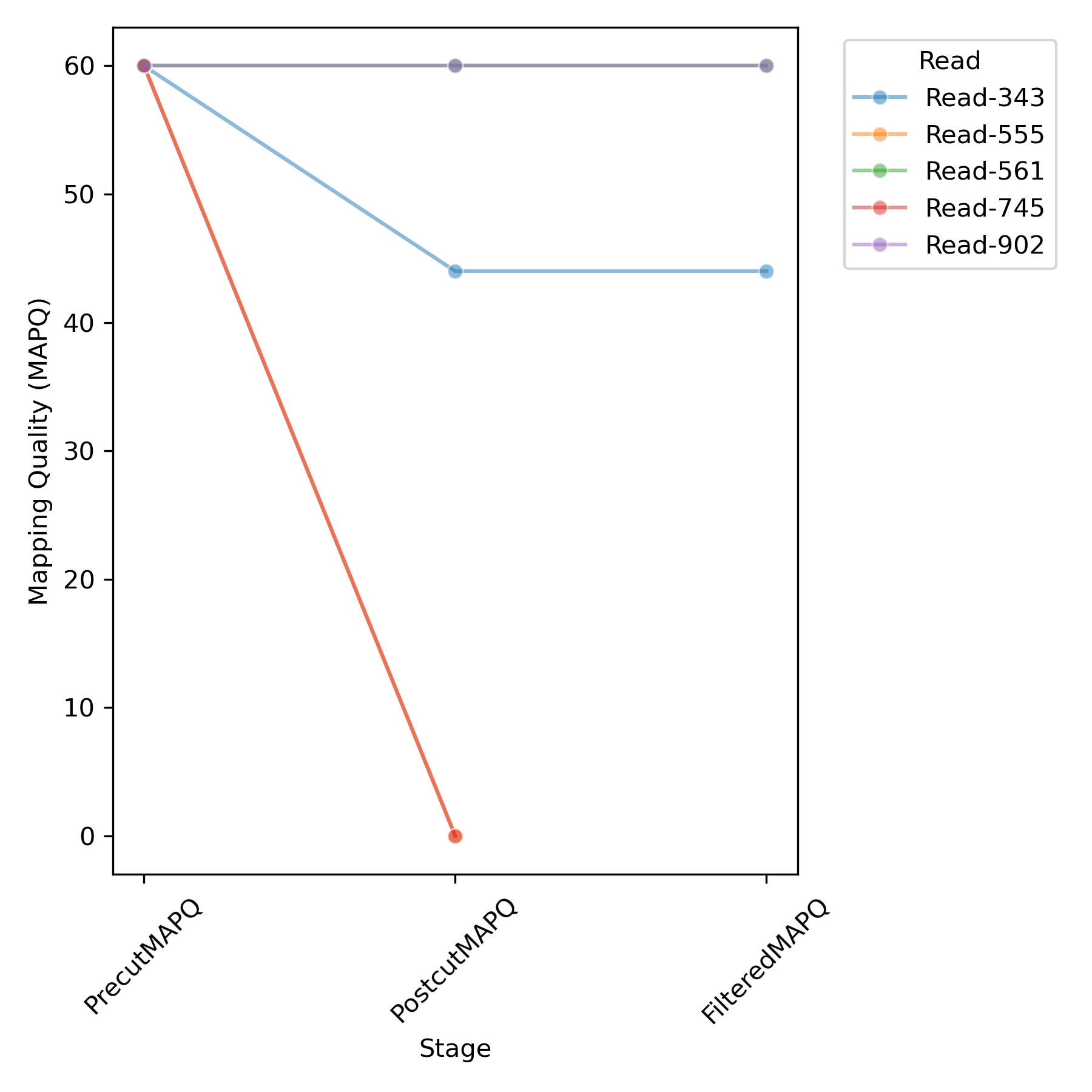
The table illustrates changes in mapping quality and chromosome alignment for each read with an insertion across three stages: Precut mapping before any modifications, Postcut mapping after the reads were modified, and Filtered mapping after filtering based on mapping quality.
Info
During the initial mapping of the unaltered reads, four out of the five reads containing detected insertions predominantly aligned with high quality to the vector reference. However, after the modification (Buffer), where every base of the insertion was replaced with N, two additional reads successfully mapped to a region in the reference genome, while the other two reads became unmappable.
Info
The scores from the table are automatically visualized in the plot. However, due to overlapping quality scores, some reads may be obscured by others with identical values. In the example data, this occurs with Read-902 and Read-561, as well as for Read-555 and Read-745.
S1:
Fragmentation
The fragmentation process is a crucial step not only for detecting insertions but also for gaining a detailed understanding of the exact composition and orientation of the inserted sequence. Some aspects of fragmentation quality control align closely with the analysis of the orientation and structure of the detected insertions.
However, the analysis of the previously mentioned output files overlooks another critical factor: The existence of fragments with significant sequence similarity to other "normal" sequences in the reference FASTA.
The pipeline includes functionality to perform a BLASTN search of the fragmented insertion sequence against a pre-built version of your reference's BLAST database. To enable this feature, simply specify the blastn_db argument in the config.yml.
Danger
The potential similarity of the insertion sequence to other sequences in your reference is particularly important when using the pipeline in conjunction with complex vector expression systems. For example, CAR T cell vector constructs (like our example vector construct ) often insert sequences partially derived from human genes.
As this option is not configured for the tutorial, we can instead rely on two other automatically generated plots to gain insights into potential false-positive matches for the insertion sequence.
Directory: ../final/qc/Fragmentation/Insertions/Insertions_{fragmentsize}_{sample}/
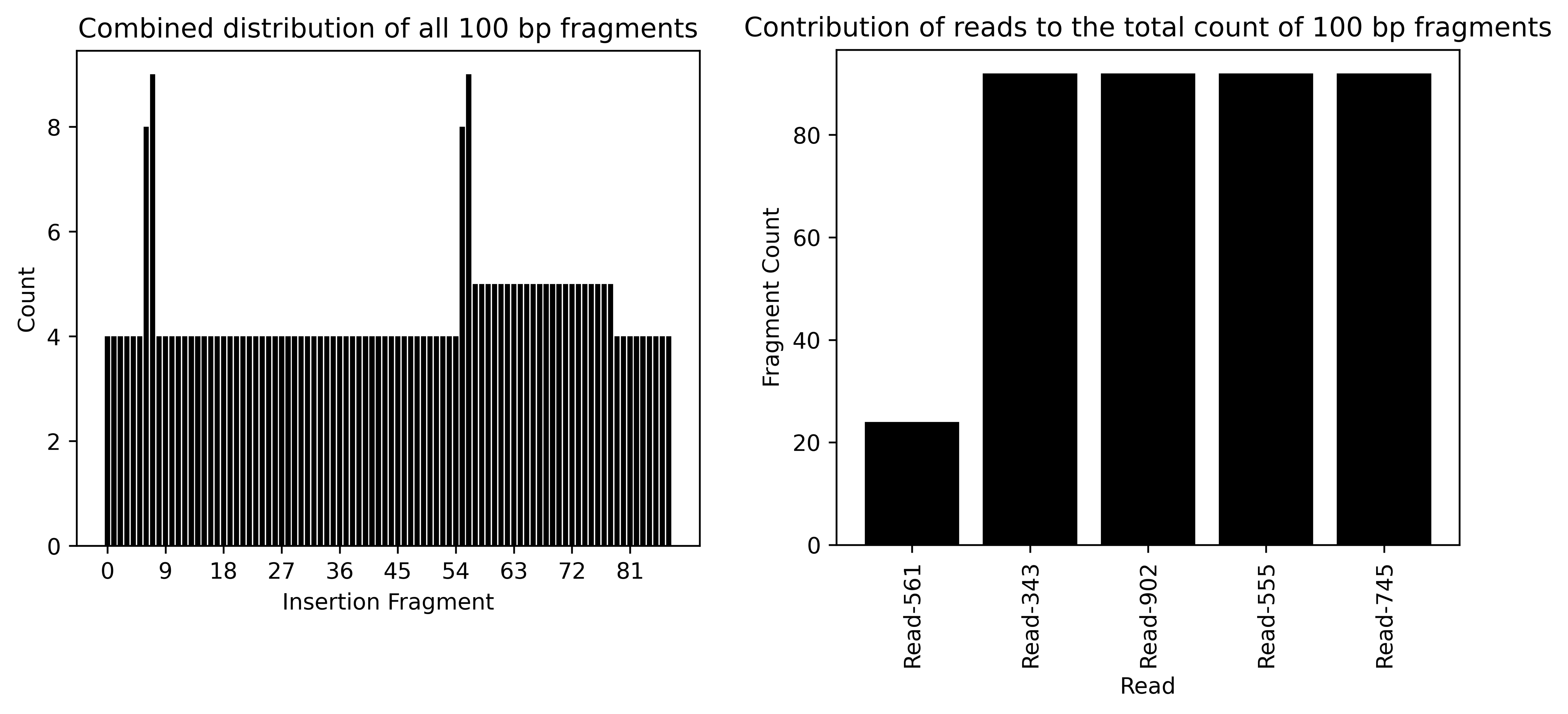
These two plots illustrate the distributions of all insertion fragments (left) and the number of fragment matches "contributed" by each read (right).
Info
The Combined distribution of all 100 bp fragments plot reveals that every fragment of the vector is represented at least four times. However, fragments 6,7,55, and 56 are noticeably overrepresented in the reads. As mentioned in the orientation and structure section, these fragments correspond to the vector's LTRs, making their alignment ambiguous. The slight plateau observed between fragments 57 and 78 is better understood in conjunction with the second plot.
The Contribution of reads to the toal count of 100 bp fragments plot clarifies this plateau by showing the read-specific contributions of fragments. Four reads contribute the maximum number of vector fragments, whereas Read-561 includes only about 21 vector fragments. This leads to the slight overrepresentation of fragments 57 to 78 in the Combined distribution of all 100 bp fragments plot.
Attention
Observations like these can help to determine the most accurate MinInsertionLength threshold in the config.yml.
Further Details
For the example data, we selected only a very small portion of the reference genome to generate reads. This is why there are no additional "off-target" fragment matches within our reads. Since the vector construct contains several human-derived components in its architecture, a real sequencing dataset would likely result in a more complex barplot.
As mentioned before, the safest way to identify potential misleading fragment matches in advance is to provide a human BLASTN reference database to the pipeline. The vector fragments are then automatically aligned against this reference, and the resulting plots offer an overview of the vector regions that are highly likely to appear, even in the absence of an actual insertion.
S1 Barplots when provided a
BLASTN reference: 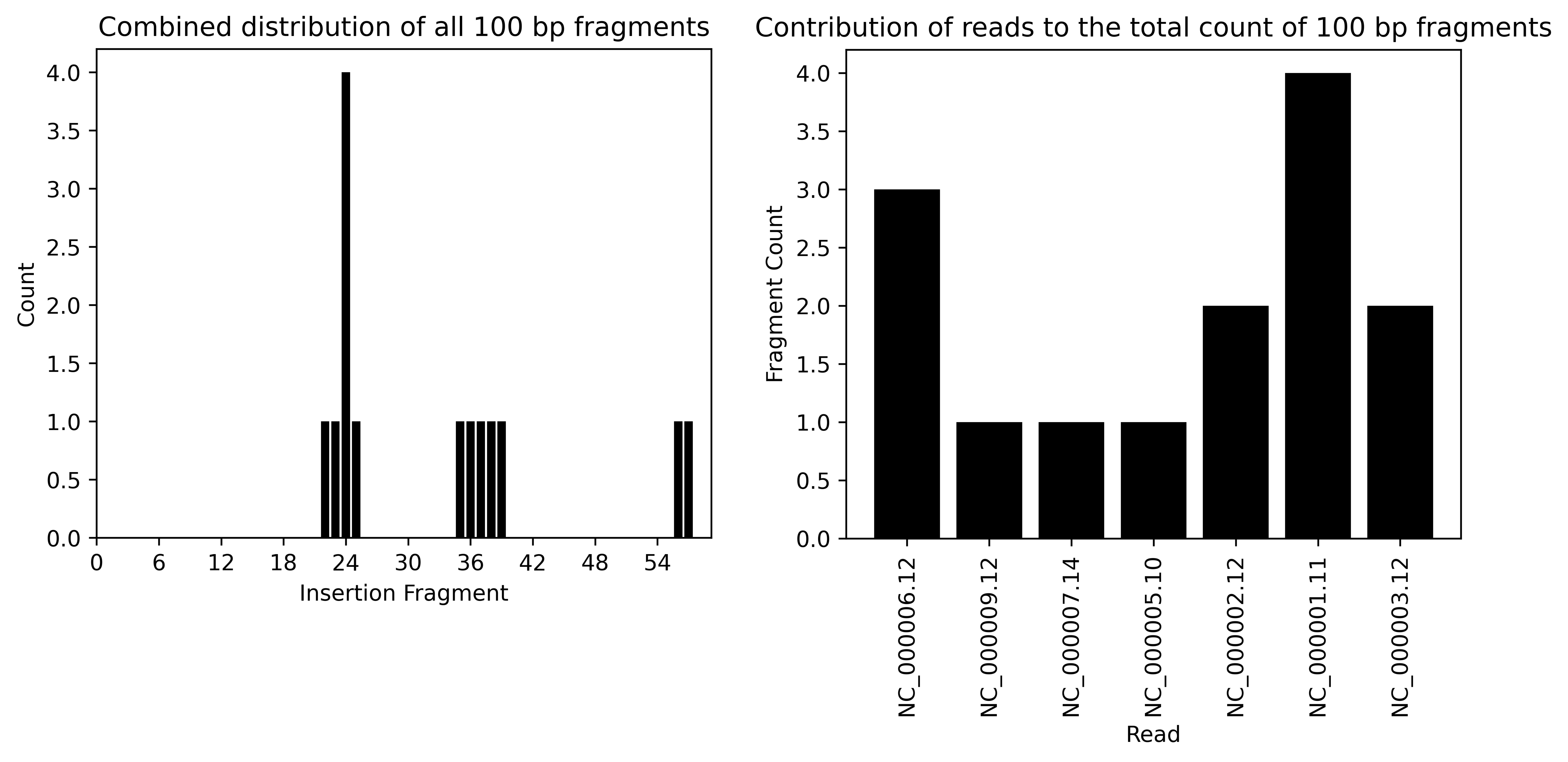
The bar plots now illustrate which vector fragments are likely to produce false positives. When comparing these fragments with the structure of the construct, you can identify three main regions of fragment matches: fragments 22–25 correspond to the EF-1a core promoter, fragments 35–39 align with CD28 and CD247, and fragments 56–57 represent the 3'LTR. These are all (to some extend) human components in the vector architecture that we can also anticipate detecting with the pipeline by using the vector genome as the target sequence.
3. Functional annotation
Typically, identifying the genomic localization of an insertion is just the starting point. A basic yet essential functionality for annotating the detected insertion sites is included in the pipeline through the functional_genomics.smk rule collection. The pipeline can work with different user-defined BED annotation files that can be provided in the config.yml as simple as annotate_{key}.
Genes in proximity
For the tutorial, we have defined only one annotation file in the config.yml, which simply contains the known genes located in our specified reference FASTA. For details on generating this file, refer to this. The pipeline compares the locations of the insertions with the entries in the provided annotation file and reports the closest match of each insertion with each annotation, thus producing the file below.
File: ../final/functional_genomics/Functional_distances_to_Insertions_{sample}.bed
S1:
| InsertionChromosome | InsertionStart | InsertionEnd | InsertionRead | InsertionOrig | InsertionStrand | AnnotationChromosome | AnnotationStart | AnnotationEnd | AnnotationID | AnnotationScore | AnnotationStrand | AnnotationSource | Distance |
|---|---|---|---|---|---|---|---|---|---|---|---|---|---|
| chr1 | 270204 | 270205 | Read-561 | [257666, 291832] | + | chr1 | 266854 | 268655 | ENSG00000286448 | . | + | annotate_ucsc_genes | -1550 |
| chr1 | 314899 | 314900 | Read-343 | [296872, 297968] | + | chr1 | 360056 | 366052 | ENSG00000236601 | . | + | annotate_ucsc_genes | 45157 |
| chr1 | 432141 | 432142 | Read-902 | [428005, 432140] | + | chr1 | 450739 | 451678 | OR4F29 | . | - | annotate_ucsc_genes | 18598 |
Info
The header above was only added to make the interpretation of the output easier. Your own output will be without the column names.
A good starting point to get familiar with the personalization of the pipeline tailored to your specific research question can be including a rule for the visualisation of this table. Check out the advanced usage for more on this.
Further Details
The reads for this tutorial are artificially generated based on the first 50kb of sequence from human chromosome 1. The regions at the beginning of chromosomes (near the centromeres and telomeres) are typically less gene-dense compared to the more gene-rich areas toward the middle of the chromosomes. This relative scarcity of coding genes also makes these regions less accessible for the integration of lentiviral-based vector systems, thus reducing the biological plausibility of our simulated data.
4. Intermediate files
The workflow generates numerous additional files beyond previously listed. Most of these files are quite easy to understand once you are familiar with the pipeline's functionality. They are typically not essential for most use cases unless debugging is required or you integrate custom downstream rules into the analysis.
Directory: ../intermediate/
Info
Here is a list of each subdirectory and a description of what to find in them:
blastn/
Filtered_Annotated_{fragmentsize}_InsertionMatches_{sample}.blastn: Results from the BLASTn searches after filteringCoordinates_{fragmentsize}_InsertionMatches_{sample}.blastn: Dictionary of the identified FASTA coordinates based on insertions in the reads -Readnames_{fragmentsize}_InsertionMatches_{sample}.txt: Names of insertion-carrying reads.ref/:BLASTNmatches of vector fragments with provided ref blastdb (empty files if noblast_dbprovided)
fasta/
fragments/: ConstructedBLASTNdatabase based on the query insertionModified_{sample}_mod.fa: Modified FASTA file of input BAM (read modification dependent onBuffer,Split, orJoin)Full_{sample}.fa: Unmodifed FASTA file of input BAMInsertion_{sample}.fa: Detected insertion sequences extacted from the readsIsolated_Reads_{sample}.fa: Isolated reads with insertions
functional_genomics/
Annotation_ucsc_genes_Insertions_{sample}.bed: Insertions with exact annotation matches (distance=0). Based onbedtools intersect.
localization/
ExactInsertions_{sample}.bed: File as in final outputSorted_InsertionPoints_{sample}.bed: Exact points of insertion (stop = start + 1)
log/
- See Error handling
mapping/
insertion_ref_genome.fa: Genome used for mapping. Consists of user-defiend reference genome and insertion reference sequence.Isolated_Reads_{sample}.bam: Isolated reads with insertionsPrecut_{sample}_sorted.bam: Unmodified reads after reference mappingPostcut_{sample}_unfiltered_sorted.bam: (Modified) reads after reference mappingPostcut_{sample}_sorted.bam: (Modified) Reads passing the quality filter after reference mappingPostcut_{sample}_sorted.bed: Genomic locations of aligned reads
qc/
fastqc/: Fastqc input and raw outputmultiqc_data/: Multiqc raw outputnanoplot/: Nanoplot raw outputmultiqc_report.html: Report as in final output